Dynamic simulation and theoretical curve of SI virus model

SI model

Parsing

Divide the population into two types, one is the susceptible, that is, the healthy population, with S for its number.
The other is an infected person, denoted by I.
That is, the total number of people in the area is N = S + I.
I infected people, encounter r individuals every day, \(\beta\) probability of infecting diseases.
The proportion of healthy people is \( \frac{S}{N}\).
Easy to multiply all the above amounts to add new infection cases every day.
So get

Ordinary differential equation

\( \frac{dI}{dt}=r\beta I\frac{S}{N} \\ \frac{dS}{dt}=-r\beta I\frac{S}{N}\)

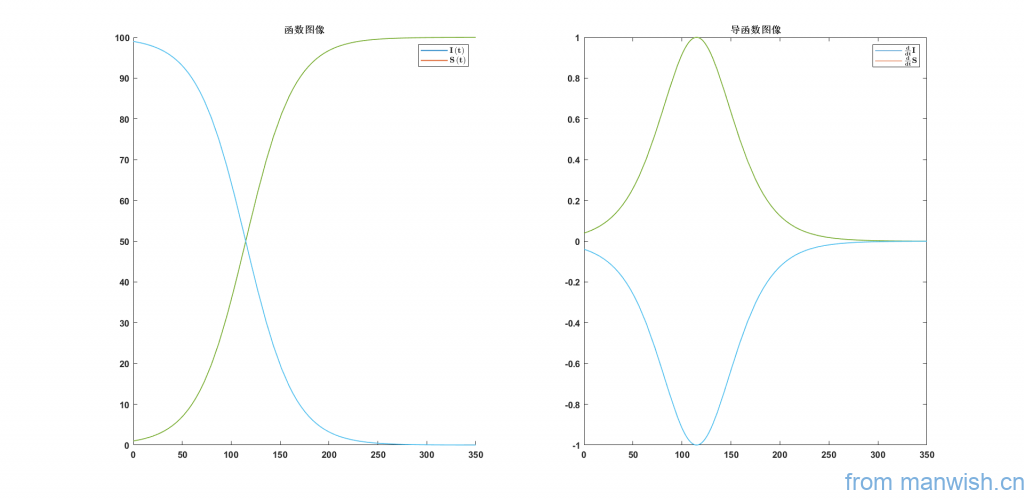
Now suppose that the total number of people is N = 100, the number of infected people contacting susceptible people r = 2, the probability of infection \( \ beta \) = 0.02, the initial infected person is 1 that is \( I\left(0\right)=1\).

Analytical solution

\( I\left(t\right)=\frac{100}{e^{\mathrm{ln}\left(99\right)-\frac{t}{25}} +1} \\ S\left(t\right)=\frac{100}{e^{\frac{t}{25}-\mathrm{ln}\left(99\right)} +1}\)

In order to observe its rate of change and derive it, we get

Derivative

\( \frac{\mathrm{d}}{\textrm{d}t}I=\frac{4e^{\mathrm{ln}\left(99\right)-\frac{t}{25}} }{{\left(e^{\mathrm{ln}\left(99\right)-\frac{t}{25}} +1\right)}^2 } \\ \frac{\mathrm{d}}{\mathrm{d}t}S=-\frac{4e^{\frac{t}{25}-\mathrm{ln}\left(99\right)} }{{\left(e^{\frac{t}{25}-\mathrm{ln}\left(99\right)} +1\right)}^2 }\)

To find the fastest growing time, find the maximum value of its derivative, ie

Fastest growth time

\(t={I^{\prime } \left(t\right)}_{\mathrm{max}} =25\,\mathrm{log}\left(99\right)\approx 115\)

Substituting into the original equation found that N = 50 at this time, in fact, the fastest growth time can be directly obtained by simple transformation.

\(\frac{dI}{dt}=r\beta I\frac{S}{N}=r\beta I\frac{N-I}{N}=r\beta I\left(1-\frac{I}{N}\right)\), so when \(I=\frac{N}{2}\) the growth is the fastest.

To analyze when everyone is infected, the derivation function is equal to zero (in fact, the mathematical model is never 0, here \(I=\frac{N}{2}\) instead)

All infected time

\(t=25\,\mathrm{log}\left(99\right)-25\,\mathrm{log}\left(1999-60\,\sqrt{10}\,\sqrt{111}\right)\approx 322\)

Illustration

General solution

Analytical solution

\( I\left(t\right)=\frac{N}{e^{\mathrm{ln}\left(-\frac{I_0 -N}{I_0 }\right)-\beta \;r\;t} +1} \\ S\left(t\right)=\frac{N}{e^{\mathrm{ln}\left(-\frac{I_0 }{I_0 -N}\right)+\beta \;r\;t} +1}\)

Derivative

\( \frac{\mathrm{d}}{\textrm{d}t}I=\frac{N\,\beta \,r\,{\mathrm{e}}^{\mathrm{log}\left(-\frac{I_0 -N}{I_0 }\right)-\beta \,r\,t} }{{{\left({\mathrm{e}}^{\mathrm{log}\left(-\frac{I_0 -N}{I_0 }\right)-\beta \,r\,t} +1\right)}}^2 } \\ \frac{\mathrm{d}}{\textrm{d}t}S=-\frac{N\,\beta \,r\,{\mathrm{e}}^{\mathrm{log}\left(\frac{N-S_0 }{S_0 }\right)+\beta \,r\,t} }{{{\left({\mathrm{e}}^{\mathrm{log}\left(\frac{N-S_0 }{S_0 }\right)+\beta \,r\,t} +1\right)}}^2 }\)

The fastest time for growth

\( t=\frac{\mathrm{log}\left(-\frac{I_0 -N}{I_0 }\right)}{\beta \,r}\)

All infected time

Set \(0={10}^{-3}\)

\(t=\frac{\mathrm{log}\left(-\frac{I_0 -N}{I_0 }\right)-\mathrm{log}\left(500\,N\,\beta \,r-500\,N\,\beta \,r\,\sqrt{\frac{250\,N\,\beta \,r-1}{250\,N\,\beta \,r}}-1\right)+2\,\pi \,k\,\mathrm{i}}{\beta \,r} \)

\( \left( \begin{align}
& {{\sigma }_{1}}\ne 1\wedge 500\,N\,\beta \,r\ne {{\sigma }_{2}}+1\wedge N\ne 0\wedge \beta \ne 0 \\
& \wedge r\ne 0\wedge {{\text{e}}^{\log \left( 500\,N\,\beta \,r-{{\sigma }_{2}}-1 \right)-2\,\pi \,k\,\text{i}}}\ne -1\wedge k\in \mathbb{Z} \\
& \text{Where} \\
& {{\sigma }_{1}}=500\,N\,\beta \,r+{{\sigma }_{2}} \\
& {{\sigma }_{2}}=500\,N\,\beta \,r\,\sqrt{\frac{250\,N\,\beta \,r-1}{250\,N\,\beta \,r}} \\
\end{align} \right)\)

View all models and notes: Infectious disease model simulation and theoretical trends

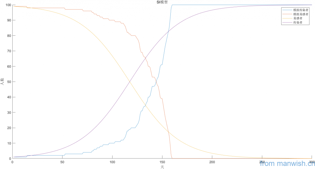
网络模拟

图示

Matlab代码

clear
figure
N = 100;    %Initial graph points
I = 1;      %Infector
Start = 20; %Starting point
r = 2;      %Number of infected persons exposed to susceptible persons
B = 0.02;   %Probability of infection
days = 300;

A=zeros(N);
Ae1=linspace(1,N,N);
Ae2=randi([1 N],1,N);
Ae3=randi([1 N],1,N);
G = graph(A);
G = addedge(G,Ae1,Ae2,1);
G = addedge(G,Ae1,Ae3,1);

[bin,binsize] = conncomp(G);
idx = binsize(bin) == max(binsize);
G = subgraph(G, idx);

G = simplify(G);
Lsg=max(binsize);
S=Lsg-I;    %Susceptible

xp=randi([0,N],1,Lsg);
yp=randi([0,N],1,Lsg);
zp=randi([0,N],1,Lsg);
p=plot(G,'Layout','force3',"NodeLabel",[]);
%p=plot(G,'XData',xp,'YData',yp,'ZData',zp,"NodeLabel",[]);
%axis([0 N 0 N 0 N])
p.NodeColor="g";
hold on

Ig = Start;
DATA=repelem(Lsg,days);
DATA(1)=I;
highlight(p,Ig,"NodeColor","red");
title('第1天')
%gif('SI-Graph.gif')
StopDay=0;
for DAY=2:days
    if length(Ig)==Lsg
        if StopDay==DAY
            break
        end
        if StopDay==0
            StopDay=DAY+30;
        end
    end
    for i=1:length(Ig)
        BFS=bfsearch(G,Ig(i));
        BFS=setdiff(BFS,Ig,'stable');
        if r>length(BFS)
            front=length(BFS);
        else
            front=r;
        end
        BFS=BFS(1:front)';
        for lp=1:front
            if rand()<=B
                Ig = [Ig BFS(lp)];
                highlight(p,BFS(lp),"NodeColor","red");
            end
        end
    end
    title(['第' num2str(DAY) '天'])
    DATA(DAY)=length(Ig);
    if rem(DAY,2)==0
        %[caz,cel] = view;
        %view(caz+1,cel)
        drawnow
        %gif
    end
end

figure
N=Lsg;
hold on
xp=linspace(1,length(DATA),length(DATA));
plot(xp,DATA,xp,Lsg-DATA)
T = 1:days;
for idx = 1:length(T)-1
    if S(idx)<0
        S(idx)=0;
    end
    if I(idx)>N
        I(idx)=N;
    end
    S(idx+1) = S(idx) - r*B*I(idx)*S(idx)/N;
    I(idx+1) = I(idx) + r*B*I(idx)*S(idx)/N;
end
a=plot(T,S,T,I);
legend('Simulated Infector','Simulate susceptible people','susceptible people','Infector');
xlabel('Day');ylabel('Number of people')
title('SI model')Code language: Matlab (matlab)

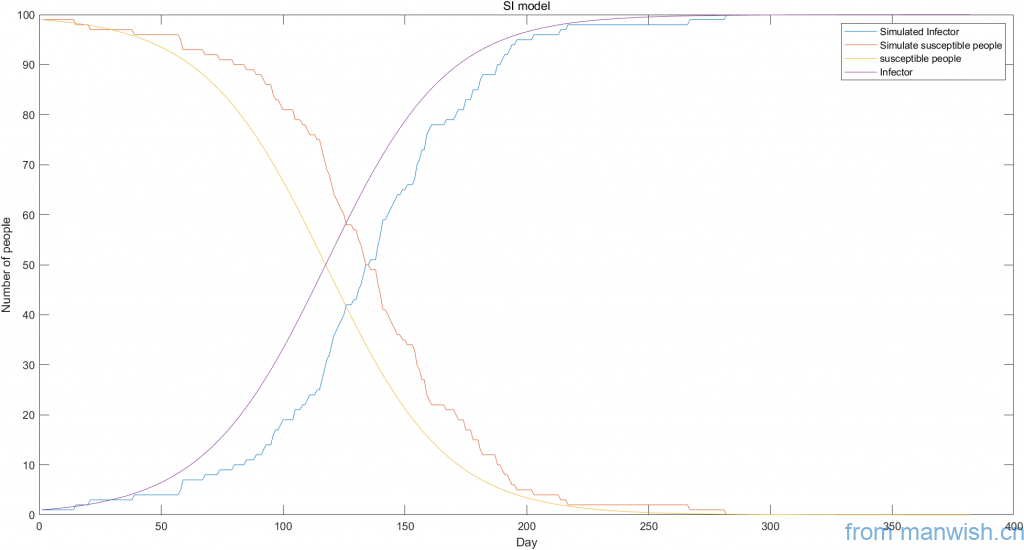
Cartesian coordinate system simulation

The final screenshot of the simulation is as follows (the dynamic process is not given):

Matlab Code

clear
figure
N = 100;      %Total population
I = 1;        %Infector
S = N - I;    %susceptible person

R = 2;        %Number of infected persons exposed to susceptible persons
B = 0.02;     %Probability of infection
days = 200;
Dynamic = false;  %Set to true to show the dynamic process

Sdata=[];

state=zeros(1,N);
index=randperm(N,I);
state(index)=1;
if Dynamic
    axis([0 N 0 N]);
    hold on
end
for i=1:days
    xpos=randperm(N);
    ypos=randperm(N);
    if sum(state)==100
        break
    end
    for j=1:N
        if state(j)~=1
            continue
        end
        dis=sqrt((xpos-xpos(j)).^2+(ypos-ypos(j)).^2);
        l=0;
        for k=1:N
            if state(k)==1
                continue
            end
            l=l+1;
            peo(l).dis=dis(k);
            peo(l).num=k;
        end
        T = struct2table(peo);
        sortedT = sortrows(T,'dis');
        sortedS = table2struct(sortedT);
        tp=sortedT{1:R,2};
        for k=1:length(tp)
            if rand()<=B
                state(tp(k))=1;
            end
        end
    end
    Sdata(i)=sum(state);
    a=-8;
    b=8;
    %xpos=xpos+ a + (b-a).*rand(1,N);
    %ypos=ypos+ a + (b-a).*rand(1,N);
    if Dynamic && rem(i,10)==0
        phd=scatter(xpos,ypos,[],state,"filled");
        title(['Day ' num2str(i)])
        drawnow
        delete(phd)
    end
end
%Display curves of simulated data and calculate theoretical data
figure
set(gcf,'visible',true)
days=length(Sdata);
plot(1:days,Sdata,1:days,N-Sdata)
hold on
T = 1:days+100;
for idx = 1:length(T)-1
    if S(idx)<0
        S(idx)=0;
    end
    if I(idx)>N
        I(idx)=N;
    end
    S(idx+1) = S(idx) - R*B*I(idx)*S(idx)/N;
    I(idx+1) = I(idx) + R*B*I(idx)*S(idx)/N;
end
plot(T,S,T,I);
legend('Simulated Infector','Simulate susceptible people','susceptible people','Infector');
xlabel('Day');ylabel('Number of people')
title('SI model')Code language: Matlab (matlab)