Infectious disease model simulation and theoretical trends

introduction

Mathematical models can project how infectious diseases progress to show the likely outcome of an epidemic and help inform public health interventions. Models use basic assumptions or collected statistics along with mathematics to find parameters for various infectious diseases and use those parameters to calculate the effects of different interventions, like mass vaccination programmes. The modelling can help decide which intervention/s to avoid and which to trial, or can predict future growth patterns, etc.[1]

Use Matlab for simulation and drawing

SI model

Divide the population into two types, one is the susceptible, that is, the healthy population, with S for its number.
The other is an infected person, denoted by I.
That is, the total number of people in the area is N = S + I.
I infected people, encounter r individuals every day, \( \beta\) probability of infecting diseases.
The ratio of healthy people is \( \frac{S}{N}\).
Multiply all of the above to add new infection cases every day.

Differential Equations

\( \frac{\mathrm{d}}{\mathrm{d}t}I=r\beta I\frac{S}{N} \\ \frac{\mathrm{d}}{\mathrm{d}t}S=-r\beta I\frac{S}{N}\)

Iterative equation

\(I_n =I_{n-1} +r\beta I_{n-1} \frac{S_{n-1} }{N} \\ S_n =S_{n-1} -r\beta I_{n-1} \frac{S_{n-1} }{N} \)

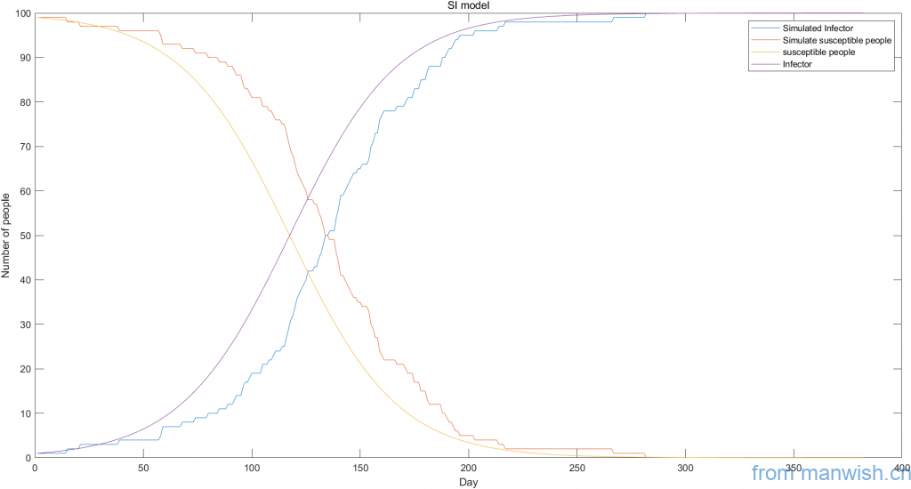
Simulation and theoretical trend graph

Matlab code

Dynamic simulation and theoretical curve of SI virus model

---

SIS model

Increase the probability of infected person I recovering health \(\gamma\).
After recovery, it may still be infected again.

Differential Equations

\( \frac{\mathrm{d}}{\mathrm{d}t}I=r\beta I\frac{S}{N}-\gamma I \\ \frac{\mathrm{d}}{\mathrm{d}t}S=-r\beta I\frac{S}{N}+\gamma I\)

Iterative equation

\( I_n =I_{n-1} +r\beta I_{n-1} \frac{S_{n-1} }{N}-\gamma I_{n-1} \\ S_n =S_{n-1} -r\beta I_{n-1} \frac{S_{n-1} }{N}+\gamma I_{n-1}\)

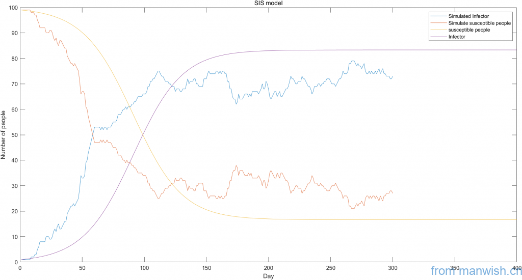
Simulation and theoretical trend graph

Matlab code

Dynamic simulation and theoretical curve of SIS virus model

---

SIR model

Introduce the rehabilitation person R and satisfy the total number N = S + I + R.
Once it becomes a recovered person, there is no chance that it will become infected or susceptible again.
In fact, the \( \gamma I\) in the \( \frac{d}{\textrm{d}t}S\) in the SIS model is taken out to assign a new differential \( \frac{d}{\textrm{d}t}R\)

Differential Equations

\( \frac{\mathrm{d}}{\mathrm{d}t}I=r\beta I\frac{S}{N}-\gamma I \\ \frac{\mathrm{d}}{\mathrm{d}t}S=-r\beta I\frac{S}{N} \\ \frac{\mathrm{d}}{\mathrm{d}t}R=\gamma I\)

Iterative equation

\(I_n =I_{n-1} +r\beta I_{n-1} \frac{S_{n-1} }{N}-\gamma I_{n-1} \\ S_n =S_{n-1} -r\beta I_{n-1} \frac{S_{n-1} }{N} \\ R_n =R_{n-1} +\gamma I_{n-1}\)

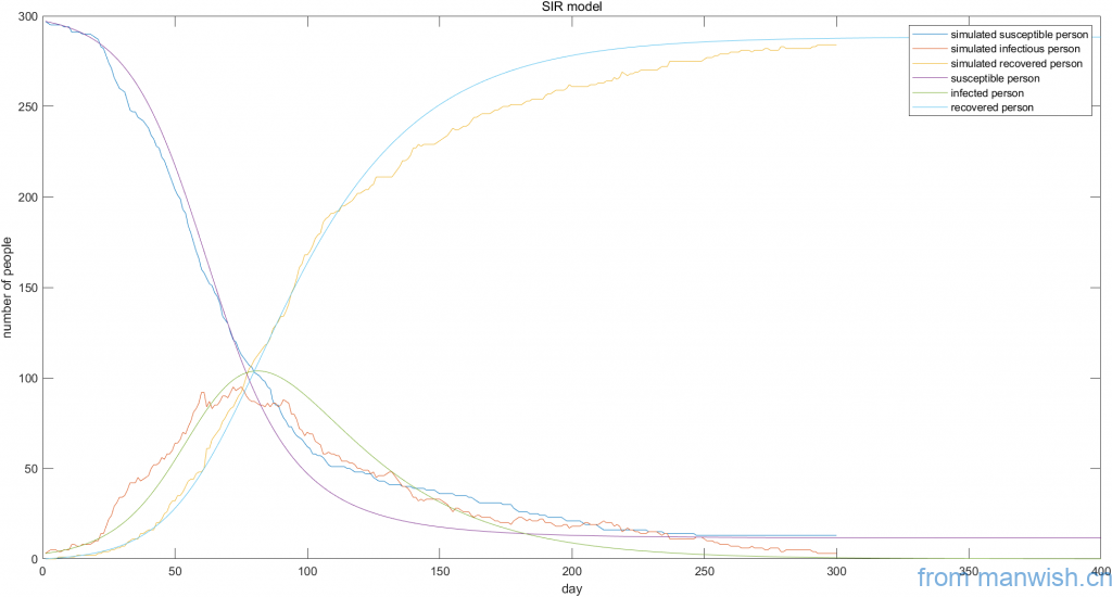
Simulation and theoretical trend graph

Matlab code

Dynamic simulation and theoretical curve of SIR virus model

---

SEIR model

People who are susceptible will experience an incubation period at first, and symptoms will not appear until some time later.
Therefore, based on the SIR model, the latent person E is introduced, and the latent person is converted into an infected person according to the probability \( \alpha\).
Intersect \( r\beta I\frac{S}{N}\) of \( \frac{d}{\textrm{d}t}I\) in the SIR model To \( \frac{d}{\textrm{d}t}E\), add \( \alpha E\) to \( \frac{d}{\textrm{d}t}E\) and \( \frac{d}{\textrm{d}t}I\).

Differential Equations

\( \frac{\mathrm{d}}{\mathrm{d}t}E=r\beta I\frac{S}{N}-\alpha E \\ \frac{\mathrm{d}}{\mathrm{d}t}S=-r\beta I\frac{S}{N} \\ \frac{\mathrm{d}}{\mathrm{d}t}R=\gamma I \\\frac{\mathrm{d}}{\mathrm{d}t}I=\alpha E-\gamma I\)

Iterative equation

\(I_n =I_{n-1} +\alpha E_{n-1} -\gamma I_{n-1} \\ S_n =S_{n-1} -r\beta I_{n-1} \frac{S_{n-1} }{N} \\ E_n =E_{n-1} +r\beta I_{n-1} \frac{S_{n-1} }{N}-\alpha E_{n-1} \\ R_n =R_{n-1} +\gamma I_{n-1}\)

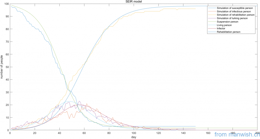
Simulation and theoretical trend graph

Matlab code

Dynamic simulation and theoretical curve of seir virus model

---

Improved SEIR model

In fact, the contact between a latent person and a normal person may also cause the normal person to become a latent person.
Therefore, the introduction of latent infection probability\(\beta_2\) can transform a healthy susceptible person into a latent person.
The number of healthy susceptible persons that the lurking person contacts every day is \(\gamma_2\).
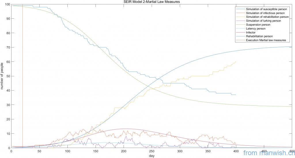
The introduction of martial law measures has reduced the number of contacts since the start of martial law (Day D).

Differential Equations

\( \frac{\mathrm{d}}{\mathrm{d}t}E=r\beta I\frac{S}{N}-\alpha E+r_2 \beta_2 E\frac{S}{N} \\ \frac{\mathrm{d}}{\mathrm{d}t}S=-r\beta I\frac{S}{N}-r_2 \beta_2 E\frac{S}{N} \\ \frac{\mathrm{d}}{\mathrm{d}t}R=\gamma I \\ \frac{\mathrm{d}}{\mathrm{d}t}I=\alpha E-\gamma I\)

Iterative equation

\( I_n =I_{n-1} +\alpha E_{n-1} -\gamma I_{n-1} \\ S_n =S_{n-1} -r\beta I_{n-1} \frac{S_{n-1} }{N}-r_2 \beta_2 E_{n-1} \frac{S_{n-1} }{N} \\ E_n =E_{n-1} +r\beta I_{n-1} \frac{S_{n-1} }{N}-\alpha E_{n-1} +r_2 \beta_2 E_{n-1} \frac{S_{n-1} }{N} \\ R_n =R_{n-1} +\gamma I_{n-1}\)

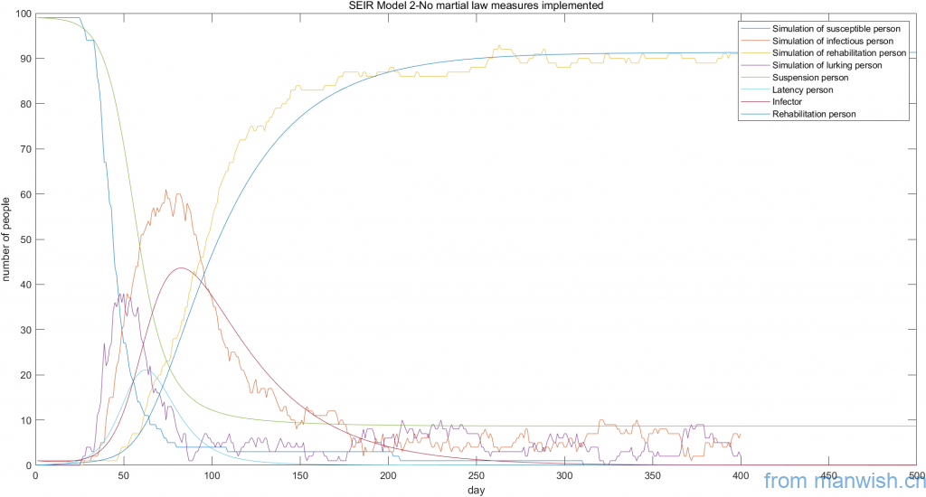
Simulation and theoretical trend graph

No isolation measures implemented

Isolation measures will be implemented on the 20th day

Matlab code

Improved SEIR virus model dynamic simulation and theoretical curve

Explanation

Please let me know if you have any errors or questions.

In the Matlab simulation code parameters, the initial number of infected persons is set to 1 to speed up the simulation. However, this will cause the first person to heal directly in the event of recovery to simulate abnormal data and run it again.